Fine-Tuning ResNet-18 for Audio Classification

Originally published as a Weights & Biases report on October 23, 2020. Reposted here for archival purposes. Code is available at github.com/jhartquist/fastaudio-experiments.

Introduction

One challenge that all ML researchers face at one point or another is hyperparameter tuning. Once the data is obtained, cleaned, and transformed, you have to choose which algorithm to apply, and most have at least a few hyperparameters that drastically affect the final results. This is especially true for deep learning: network architecture, learning rate, batch size, number of epochs, and many others. Trying every combination is expensive in both time and resources.

Even when many experiments are run, usually only the best results get reported, and it isn't always clear which hyperparameters were used or how many configurations were tested. While it's becoming more common for researchers to publish their code, tools like Weights & Biases (the platform I'm writing this report on) bring even more transparency and reproducibility to ML research. You can visualize a single training run, compare statistics across many runs, and save the exact code and parameters used for each one.

I decided to apply it to a problem I'm already familiar with. About two years ago, I wrote a blog post about using PyTorch and fastai to generate spectrograms for audio classification at training time. Since then, fastai v2 has been released, and a module called fastaudio was created to streamline the whole process. The fastaudio creators also set up a small competition repository based on the ESC-50 dataset, a collection of 2000 audio samples labeled with 50 classes. I thought it would be fun to train baseline models and try to beat some existing benchmarks (86.50% was the highest listed at time of writing).

The general fastaudio approach is to transform raw audio into log-mel spectrograms — two-dimensional, image-like representations — which can then be fed to traditional computer vision models. Since the audio-to-spectrogram conversion has its own hyperparameters (window size, hop length, number of mels, FFT size, etc.), I figured it would be useful to see how each one affects classification accuracy. As an example, this paper increased accuracy on their task from 88.9% to 96.9% just by adjusting spectrogram parameters. Since ESC-50 is small, you can train a decent model in a few minutes, making it ideal for running many experiments.

The Experiment

Experiment Setup

The goal was to determine how varying each spectrogram parameter affects classification accuracy. After some initial experiments, I focused on the transfer learning case and fine-tuned pre-trained ResNet-18 models on image-like spectrograms. While spectrograms are different from real images in many ways, I achieved pretty good accuracy in a short amount of time. Training models from scratch took 3-4× as long to reach similar accuracy.

Data

I used the ESC-50 dataset, which comes with its own cross-validation splits. For all hyperparameter experiments, I used fold 1 as the validation set. At the end, once I found a good combination, I ran many trials using each fold as the validation set in turn to report the final mean accuracy.

Tools

I used the new version of fastai along with fastaudio to train the models, and W&B to track each run. Fastai makes the integration easy — just add a callback to the Learner object. The "Sweep" feature of W&B was especially useful: define which parameters to vary, then turn on one or more agents to train a model for every combination (grid search). I rented a cloud GPU server from DataCrunch.io with 8× V100 GPUs for about 24 hours and trained 1,430 models in total.

Reproducibility

When training deep learning models, you generally get varying results even with identical hyperparameters, due to randomness from weight initialization and data shuffling. Fastai comes with a set_seed function that sets seeds for numpy, pytorch, and random, so each run can be reproduced exactly. The wandb Python client also has a save_code parameter that, when enabled at init time, saves the script or notebook alongside the training stats. If run from a git repository, it also saves the commit hash and any sweep parameters.

Training Script

All the code is in train.py and utils.py in the associated GitHub repo. At the top of the script, default parameters are passed to wandb.init:

run_config = dict(
    # spectrum
    sample_rate=44100,
    n_fft=4096,
    n_mels=224,
    hop_length=441,
    win_length=1764,
    f_max=20000,
 
    # model
    arch='resnet18',
 
    # training
    learning_rate=1e-2,
    n_epochs=20,
    batch_size=64,
    mix_up=0.4,
    normalize=True,
 
    # data
    trial_num=1,
    fold=1,
)

A sweep configuration file can then replace specific parameters across many runs. For example, to test multiple batch sizes:

program: train.py
method: grid
project: fastaudio-esc-50
parameters:
  batch_size:
    values: [8, 16, 32, 64, 96, 128, 192, 256]

To run each configuration multiple times, I added a trial_num parameter so each batch_size was run for each distinct value, averaging over 5 trials. The following produces 40 total runs:

parameters:
  batch_size:
    values: [8, 16, 32, 64, 96, 128, 192, 256]
  trial_num:
    values: [1, 2, 3, 4, 5]

Hyperparameters Tested

For more on spectrogram parameters, I highly recommend the YouTube series Audio Signal Processing for Machine Learning by Valerio Velardo. For this experiment, I ran a sweep for each of:

• hop_length — number of samples between consecutive analysis frames
• win_length — number of samples in the analysis window
• n_mels — number of mel frequency bands
• n_fft — size of the FFT computed on the window before converting to mel bands
• f_max — frequency upper bound used to create mel bands
• normalize — whether the mel spectrogram output is normalized to mean 0, std 1
• mix_up — amount of MixUp used during training
• n_epochs — number of epochs to fine-tune for
• batch_size — size of the training batch

I averaged results over 5 trials per sweep and tested each configuration at 10, 20, and 80 epochs. In all cases I used the default learning rate of 0.01, and the results below correspond to the 80-epoch versions unless otherwise specified. I also used a sample rate of 44,100 Hz, the rate of the raw audio.

Sweep Results

hop_length

Hop length is measured in samples here, and 441 samples corresponds to 10 ms at 44,100 Hz. A hop_length of 308 samples (about 7 ms) had the highest average accuracy overall, while 529 produced the lowest validation loss. Hop length is important because it directly affects how "wide" the spectrogram image is — a hop_length of 5 ms might give slightly higher accuracy than 10 ms, but the images will be twice as large and take twice as much GPU memory.

win_length

When generating a spectrogram with most audio libraries, if the window length isn't set, it defaults to the FFT size. Usually FFT size is set to a power of 2 because it's computationally more efficient (though this isn't necessarily the case depending on the implementation). The window length cannot be larger than the FFT size, but if shorter, the FFT buffer is zero-padded. It's a very important parameter for the time-frequency tradeoff: smaller windows give good time resolution but poor frequency resolution (especially in the low frequencies); larger windows give good frequency resolution but average over a longer period.

In this sweep, 2205 samples (50 ms) produced the best average accuracy, though I was surprised that 4410 (100 ms) was almost as good.

n_mels

If hop_length determines the width of the spectrogram, n_mels determines the height. After producing a regular STFT with an FFT size of, say, 2048, the result is a spectrum with 1025 FFT bins varying over time. When converting to a mel spectrogram, those bins are logarithmically compressed down to n_mels bands. This sweep showed that 32 is too few, but other than that the value doesn't affect accuracy much. 128 (the fastaudio default) gave the highest mean accuracy; 160 gave the lowest mean validation loss. I'm curious whether a larger network might be able to take advantage of more mel bands.

n_fft

FFT size is an interesting parameter. At first glance, it might not be obvious why it would make a difference as long as it's larger than win_length — however many frequency bins are created get compressed to n_mels anyway, so it doesn't directly affect the shape of the spectrogram.

I believe the reason has to do with how mel bands are constructed. Lower frequency mel bands are generated from a small number of FFT bins; higher mel bands are generated from many. When you use a higher n_fft while keeping win_length the same, you don't get any more information from the raw signal — the FFT buffer is just zero-padded. But the resulting frequency spectrum is interpolated, spreading the same information across more FFT bins. When the mel bands are created (especially the low frequency ones), they get a more accurate representation because they're averaged over more values.

In this sweep I set win_length to 1024, and we see over 4% improvement in classification accuracy moving from n_fft 1024 to 4096. Beyond that, increasing n_fft further doesn't help. I believe this is the single greatest finding throughout this experiment, and it helps explain why I was able to exceed some of the public benchmarks on ESC-50.

f_max

When converting from a regular spectrogram to a mel spectrogram, you can specify f_min and f_max to define the frequency range that the bands will span. f_min defaults to 0, which I used in all cases. f_max defaults to the Nyquist frequency (half the sample rate). It's common to downsample audio to 16 kHz to minimize memory and speed up preprocessing, but if you choose hop_length and win_length in fixed time intervals (milliseconds rather than samples), the resulting spectrogram size stays the same. Using a higher sample rate lets you use a higher f_max — say 22.5 kHz at 44.1 kHz sampling, vs. only 8 kHz at 16 kHz. Whether you care about high-frequency content depends on the data.

In this dataset, lower f_max correlated with lower accuracy, but not very definitively. 18,000 Hz had the lowest validation loss on average.

normalize

When doing transfer learning with fastai, the data is normalized using the same statistics the model was originally trained on. The output of a spectrogram is significantly different from a normal image. Chris Kroenke wrote a great article about normalizing spectrograms, and I borrowed his code for this sweep — specifically the "Global Normalization" technique. My results match his: a clear improvement in both validation loss and accuracy when normalizing the data to mean 0, std 1.

mix_up

I hadn't heard of MixUp until experimenting with the baseline tutorials in the fastaudio Audio-Competition repo. It's a data augmentation technique that can significantly improve classification accuracy. Since fastai has a built-in implementation, I was able to use it with a single line of code, and it clearly helped. This is the only data augmentation in the entire set of experiments, and a value of just 0.1 produced the highest accuracy and lowest validation loss.

batch_size

The standard recommendation is to use as large a batch_size as possible without running out of GPU memory. Here, because the dataset is so small (only 2000 examples), 64 turned out to be the best value. This may be because there are more steps per epoch with a smaller batch.

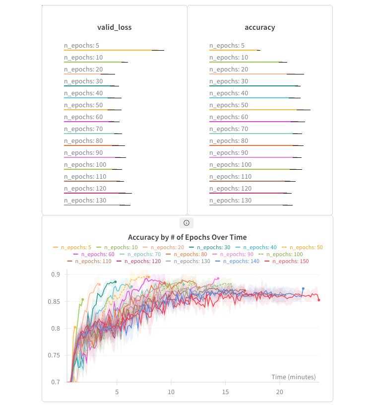
n_epochs

I ran all the previous configurations at 10, 20, and 80 epochs. While 80 was almost always better than 20, the difference wasn't huge. Because fastai uses one-cycle training by default (Leslie Smith's paper), good accuracy is sometimes possible with very few epochs, and running longer doesn't necessarily help.

In this sweep, 20 epochs produced the lowest validation loss, 50 epochs achieved the highest accuracy, and training for 150 epochs over 23 minutes was actually worse than training for 20 epochs in only 3.5 minutes.

Architecture

Now that I had a good idea of how various hyperparameters affected ResNet-18, I wanted to see what gains were possible by simply swapping out the pre-trained model for something more powerful.

As we increase the size of the ResNet model, training loss gets better all the way to ResNet-152. Validation loss is best with ResNet-34 and gets worse with ResNet-50 and ResNet-101 — possibly a sign of overfitting. The larger models may also need more training time given their parameter counts. It's also worth noting how much longer the larger models take to train at the same batch size.

We see a similar pattern with DenseNet, with DenseNet-161 performing best of all the architectures, achieving an impressive 91.4% accuracy.

Final Results

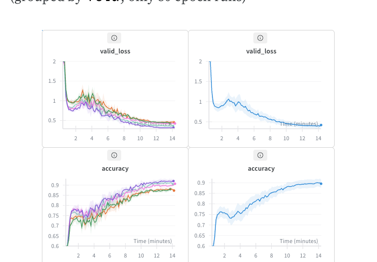
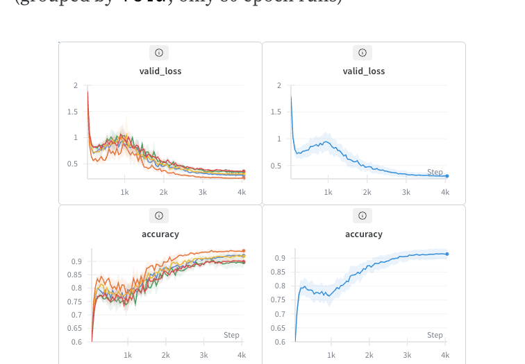
To wrap up, I measured the accuracy of a single set of hyperparameters on both resnet18 and densenet161. For each, I ran 5 trials per fold across the 5 folds and averaged the results.

resnet18

For the resnet18 trial, I averaged 25 runs each at 10, 20, and 80 epochs (75 runs total). The sweep configuration:

program: train.py
method: grid
project: fastaudio-esc-50
parameters:
  batch_size:
    value: 64
  sample_rate:
    value: 44100
  hop_length:
    value: 308
  win_length:
    value: 2205
  n_mels:
    value: 224
  n_fft:
    value: 4096
  normalize:
    value: True
  mix_up:
    value: 0.1
  f_max:
    value: 18000
  arch:
    value: resnet18
  n_epochs:
    values: [10, 20, 80]
  trial_num:
    values: [1, 2, 3, 4, 5]
  fold:
    values: [1, 2, 3, 4, 5]

Even at only 20 epochs (just under 4 minutes), we get 86.14% accuracy. For comparison, the highest accuracy listed on the official ESC-50 was 86.5%. At 80 epochs, we reach 89.54% in a little over 14 minutes. That's pretty good for a model pre-trained on images, with no data augmentation other than MixUp.

densenet161

The best results overall come from the same parameters with DenseNet-161. Averaged over 5 runs for each of the 5 folds at 80 epochs each, we see an average accuracy of 91.47%.

Conclusion

After training 1,430 models and analyzing the results with W&B, I was able to find hyperparameters that fine-tune a ResNet-18 (pre-trained on image data) to reach 89.5% accuracy in under 4 minutes, and a DenseNet-161 to 91.47%. I expect that more specialized models informed by domain expertise could go even higher with similar spectrogram settings.

Throughout this project I learned a lot about both designing experiments and training deep learning models. I'm grateful for the open-source libraries and communities that make this kind of research both possible and accessible. Future directions include applying these techniques to larger audio classification datasets and comparing different audio-domain data augmentation strategies.

Links

• Experiment repo
• fastai
• fastaudio
• Original blog post on generating spectrograms during training
• ESC-50 dataset
• MixUp paper
• One-cycle learning rate paper
• Spectrogram normalization article
• DataCrunch
• Audio Signal Processing for Machine Learning — Valerio Velardo's YouTube series