Resonators: A Rust Port of the Resonate Algorithm
Last week I published my first open source library named resonators. It's an implementation of Alexandre François' Resonate algorithm for real-time spectral analysis written in Rust and includes bindings for both Python and JavaScript (by way of WebAssembly). In this post I'll cover why I built it and detail some of the learnings I've had along the way.
What is a spectrogram?
When training machine learning models on audio, it's common to first transform the signal into an image-like representation called a spectrogram. Raw audio is most commonly stored as a 1-dimensional sequential array of numbers between -1 and 1 (mono is a single array, stereo signals are stored as 2 arrays, one channel for the left speaker, and one for the right). The Fourier transform allows us to analyze which frequencies are present in the signal in a given window of time. If we slide a small window forward in time, we're able to "see" how the signal's frequency content changes through time. This is known as the Short-Time Fourier Transform (STFT). For a deeper visual intuition on signals and the Fourier transform, Jack Schaedler's Circles, Sines, and Signals is a great interactive primer.
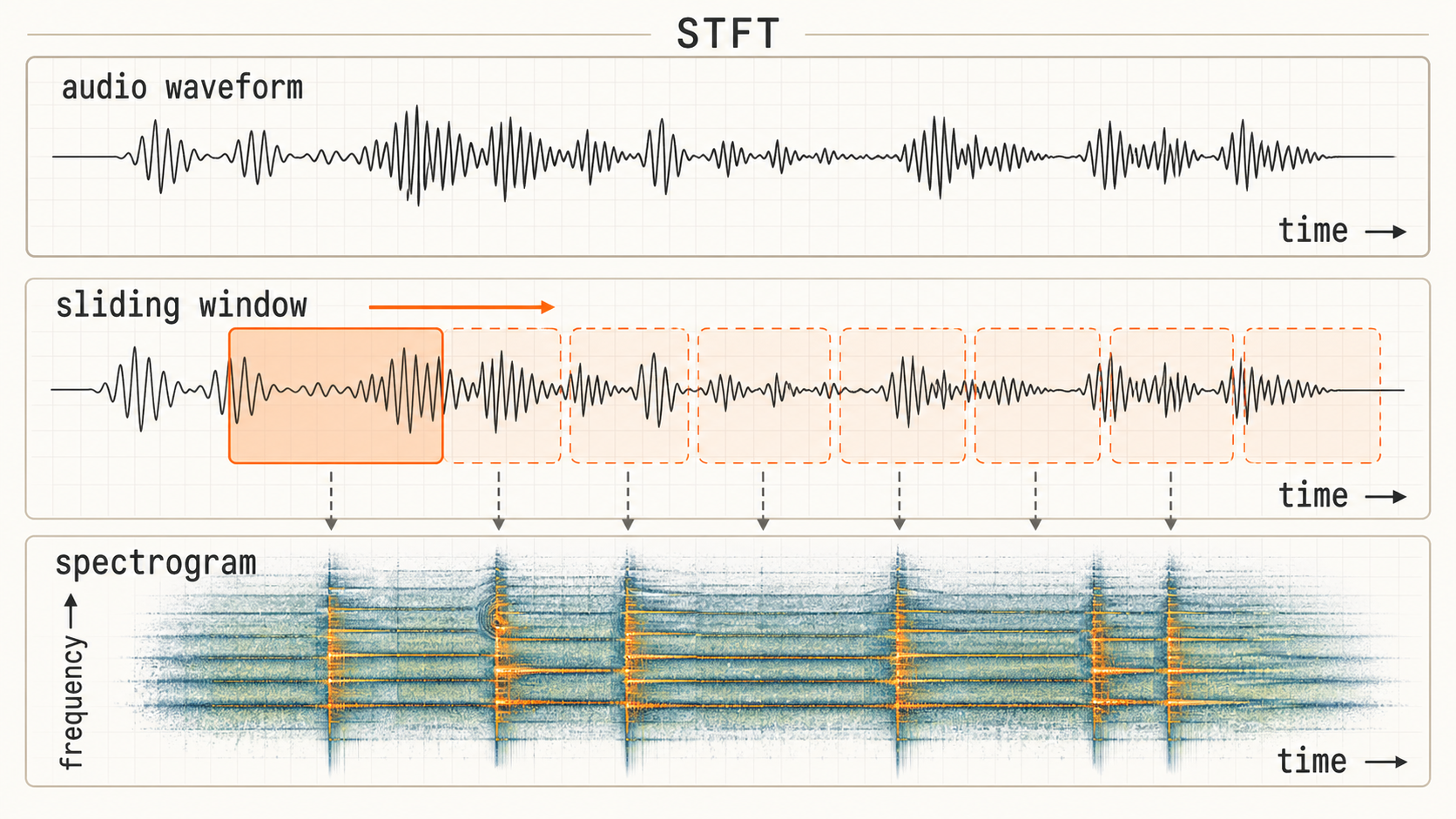
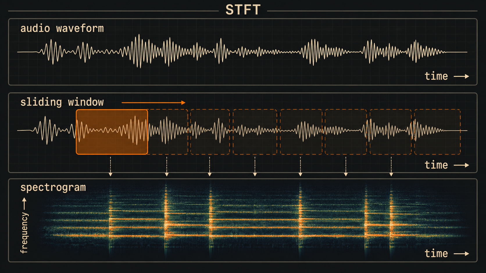
Machine learning models are very good at analyzing patterns in these images for tasks such as classification or in the case of music transcription models, pitch detection. The Fast Fourier Transform, or FFT, is an extremely efficient algorithm for calculating the Fourier transform, making it feasible to run at real-time speeds. The standard STFT comes with a time-frequency tradeoff due to the fact that it uses a fixed-size sliding analysis window. If this window is very long, say, 1 second, we get very fine frequency resolution. We may be able to detect a specific piano note, but we don't know precisely when in that second it occurred. Conversely, with a very short window, say 5ms, we get very fine time resolution, good for, say, detecting drum beats, but not as much information about which frequencies were present. One common approach is to take a "medium" sized window, maybe 2048 samples, and move it forward at a "hop size" of 512 samples.
The FFT returns frequency information in discrete bins, each of which is spaced by a fixed bandwidth. For example, depending on the window and FFT size, we might have information for frequencies at 5 Hz, 10 Hz, 15 Hz, 20 Hz, etc. If there was a sine wave at 100 Hz and another at 150 Hz, we would see two peaks in the magnitude spectrum. If instead the two sine waves were at 100 Hz and 101 Hz, we would only see a single peak at the 100 Hz bin. The 5 Hz bin width would be insufficient to tell these two components apart.
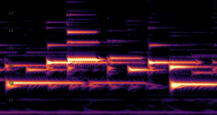
This is suboptimal for musical signals particularly, because we hear pitch on a logarithmic scale. The two lowest keys on the piano are A0 at 27.5 Hz and A#0 at 29.1 Hz, less than 2 Hz difference. Contrast that with the highest notes on the piano, B7 at 3951.1 Hz and C8 at 4186 Hz, more than 100 times the difference. Evenly spaced bins are a poor fit: the low notes could use more bins than they get, and the high notes have plenty to spare.
The Constant-Q Transform
What we would prefer is to have bins spaced more like pitch, and that's exactly what the Constant-Q Transform (CQT) provides: logarithmically spaced bins, each with a different effective window size (calculated from its frequency and a constant named Q). This turns out to work well for music models, and is used in Spotify's polyphonic transcription model Basic Pitch, which contains fewer than 17k parameters (tiny as far as deep learning models go). Unfortunately, CQT has a few drawbacks that make real-time deployment challenging. Like the STFT, it relies on a sliding window, so input must be buffered every HOP_SIZE samples. Computing the CQT is somewhat complex, and often requires computing multiple FFTs at different sample rates. Finally, while Q defines the time-frequency tradeoff, it still applies to every bin, so we can't tune it for low frequencies without also affecting the high frequencies.
The Resonate algorithm
Alexandre's Resonate algorithm fixes many of these issues. It consists of multiple "resonators", which act like independent tuning forks, each with their own target frequency. As input audio arrives, every sample updates each resonator. There is no sliding analysis window or block-level input buffering required. Each resonator stores a few floats of state and a small per-sample update, and no FFTs are involved. Furthermore, each resonator can specify how long its "time window" is by deciding how much to weight each new sample update, effectively controlling how quickly old energy decays. This means that each bin's time-frequency tradeoff can be set independently, with very low latency. With CQT or STFT, if we wanted to halve the HOP_SIZE, we'd have to do double the work computing FFTs. With resonators, we can simply read the current values twice as often, because they're being updated constantly.
Why I built it
The reference implementation, noFFT, is written in C++ and provides Python bindings. It depends on Apple's Accelerate framework and is only able to run on Apple hardware, albeit very fast. As I've been training models for real-time transcription, I needed something that could run on my deep-learning desktop rig (Ubuntu) for model training, and also in the browser (for real-time inference). Porting the algorithm to Rust allowed me to implement an optimized version that runs cross-platform, with bindings for both Python and JavaScript/WASM.
maturin and PyO3 together with the numpy crate make it easy to wrap the underlying Rust implementation and return results as numpy arrays, the standard for Python data science libraries (ML framework agnostic). On the JavaScript side, wasm-bindgen handles the type marshaling between WASM and JavaScript, and helps convert final data to Float32Array (JavaScript's typed array for 32-bit floats). wasm-pack generates the minimal JavaScript glue code as well as TypeScript type definitions, ready for publication as an npm package.
Once I had the core algorithm working and verified against the reference implementation, I used cargo bench and criterion to measure performance, and gradually optimized it. I learned that by structuring the code with well-defined loops and using #[inline] in the right places, the Rust compiler (and LLVM) is able to use auto-vectorization and take advantage of SIMD to speed things up, all without depending on any external crates. In the end, I was able to get the algorithm running natively at approximately 1.6x the speed of the reference implementation on my MacBook Pro M2 Max.
In the browser
In order to measure the speed of the WASM version, I built a small web app to run benchmarks in the browser. Enabling target-feature=+simd128 for the WASM target sped things up quite a bit, but I was still leaving some performance on the table. Within 24 hours of open-sourcing the crate, @pengowray diagnosed a few remaining bottlenecks that led to an additional 14x speedup. Interestingly, the browser demo runs faster on my iPhone 16 Pro than on my MacBook Pro.
Web Audio processes sound in fixed 128-sample chunks, giving the browser 2,667 μs to deliver each one at 48 kHz. The % budget column below shows how much of that window each ResonatorBank size consumes on my MacBook Pro M2 Max:
| bins | ns / sample | μs / quantum | % budget |
|---|---|---|---|
| 88 | 60 | 8 | 0.29% |
| 264 | 143 | 18 | 0.69% |
| 440 | 236 | 30 | 1.13% |
| 880 | 475 | 61 | 2.28% |
Even at 880 resonators, the algorithm uses just over 2% of the audio thread's time, which leaves plenty of headroom for ML inference or other audio processing.
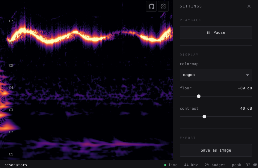
I also created a real-time spectrogram demo that analyzes microphone input (partially inspired by calebj0seph/spectro). It displays a streaming view of a CQT-like spectrum (logarithmically spaced bins), with the ability to tweak some of the settings or save as an image. It's built on the Web Audio API and updates the spectrum every 128 samples (the chunk size browsers provide). It uses a WebGL fragment shader and runs smoothly on both desktop and mobile.
Usage
The README has full setup details, but the API mirrors across all three languages:
Rust
use resonators::ResonatorBank;

let freqs = [110.0, 220.0, 440.0, 880.0];
let mut bank = ResonatorBank::from_frequencies(&freqs, 44_100.0);
let spectrogram = bank.resonate(&signal, 256);
Python
import numpy as np
from resonators import ResonatorBank

freqs = np.array([110, 220, 440, 880], dtype=np.float32)
bank = ResonatorBank(freqs, 44_100.0)
spectrogram = bank.resonate(signal, hop=256)
JavaScript
import init, { ResonatorBank } from "resonators";
await init();

const freqs = new Float32Array([110, 220, 440, 880]);
const bank = new ResonatorBank(freqs, 44100);
const spectrogram = bank.resonate(signal, 256);
resonators is just the first step of a broader exploration into real-time music analysis with ML. In the next post I'll be detailing how to feed resonator output directly into machine learning models that run in the browser, all with the core pipeline written in Rust.
Big thanks to Alexandre R. J. François for the Resonate algorithm (Best Paper at ICMC 2025) and the noFFT reference implementation. And to @pengowray for the WASM SIMD diagnosis.
resonators is open source, available on crates.io, PyPI, and npm. Source on GitHub. Licensed MIT OR Apache-2.0.